Lab 2: Strain and stress transformations
The objectives of this lab are to:
- transform 2nd Piola-Kirchhoff stress tensor components to Cauchy tensor components.
- transform stresses and strains between reference spatial and material (fibre) coordinates.
The deformations that will be considered in this lab include uniaxial deformation and equi-biaxial extension of a unit cube.
Revision
Before starting this lab, please be sure to have completed Lab 1: Analysing deformation in isotropic materials.
Section 1: Transforming from 2nd Piola-Kirchhoff to Cauchy stress tensor components
- Start OpenCMISS and load the “Kinematics analysis” project. Select “Model 1 (Uniaxial extension of unit cube)” from the drop down menu and click the “Run” button.
- Open the simulation results pane and use the components of the 2nd Piola-Kirchhoff stress tensor \((\boldsymbol{T})\) and the deformation gradient tensor \((\boldsymbol{F})\) to determine the Cauchy components of the stress tensor \((\boldsymbol{\Sigma})\) (Don’t forget the Jacobian \((J)\)). See this link for an example on how to open the simulation results pane.
Note
Hint: See equations in Section 3.1 of Nash and Hunter (2007).
- Select “Problem” from the menu bar and repeat step 1-2 for the remaining models in the kinematics analysis project.
Note
By the end of this section you should be able to:
- derive the Cauchy stress tensor components from the second Piola-Kirchhoff stress tensor components using the deformation gradient tensor.
Section 2: Transforming stresses between rotated coordinate systems
Uniaxial extension of a unit cube
- Consider the uniaxial deformation shown in the figure below, where a set of material axes are aligned with the spatial reference axes. In the following figure, the gold arrows represent the first material axis (for example, this might be a the orientation of a collagen fibre within tissue):
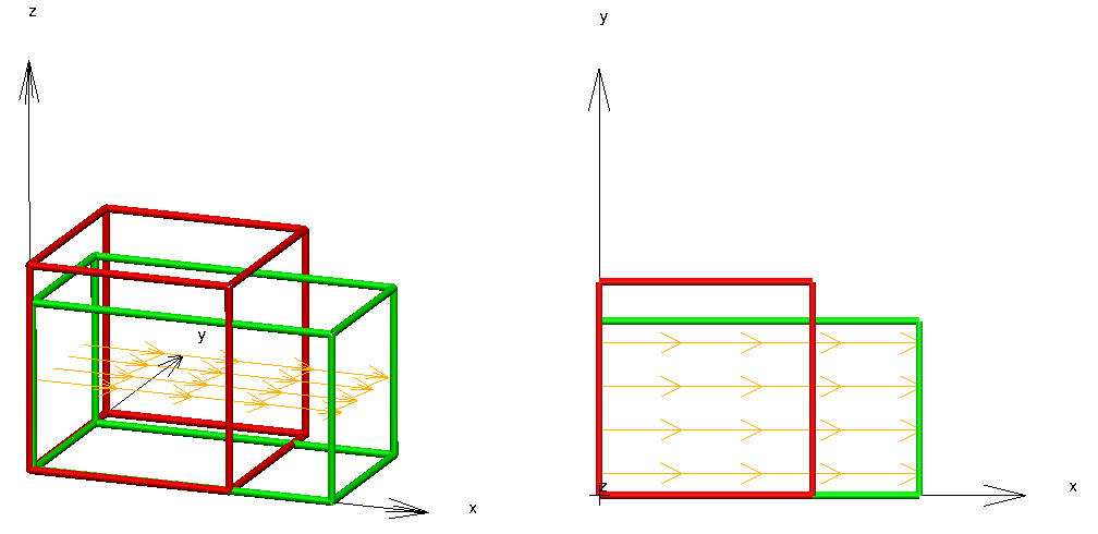
- In the screenshot:
- the undeformed (reference) configuration of the object (a unit cube) is shown in red;
- the deformed (current) configuration of the object is shown in green; and
- the gold arrows indicate the direction of the first material (fibre) axis in the object. In general, the microstructural fibres are not necessarily parallel to the direction of stretch or load.
This deformation is described by the following equations:
\[x_1 = \frac{3}{2}X_1 ~~~~ x_2 = \sqrt{\frac{2}{3}}X_2 ~~~~ x_3 = \sqrt{\frac{2}{3}}X_3\]In all figures, \(x\) represents \(X_1\) and \(x_1\), \(y\) represents \(X_2\) and \(x_2\), and \(z\) represents \(X_3\) and \(x_3\).
- Write down (see Lab 1):
- the deformation gradient tensor, \(\boldsymbol{F}=\frac{\partial\boldsymbol{x}}{\partial\boldsymbol{X}}\)
- the right Cauchy-Green deformation tensor, \(\boldsymbol{C}\) and
- the Green-Lagrange strain tensor. Label this as \(\boldsymbol{E}_{ref}\) (to indicate that it is defined with respect to the reference spatial coordinates).
Note
This is the same deformation used in Model 1 in Lab 1, so you should not need to re-do these calculations.
For this particular model, the second Piola-Kirchhoff stress tensors with respect to both the reference spatial, and material fibre axes, are:
\[\begin{split}\boldsymbol{T_{ref}} = \boldsymbol{T_{fib}} = \begin{bmatrix} 440.5 & 0 & 0 \\ 0 & 0 & 0 \\ 0 & 0 & 0 \end{bmatrix}\end{split}\](Note: While the uniaxial deformation in Model 1 of Lab 1 is the same as that considered here, the stress tensors are different between thse two labs because different stress-strain constitutive relations have been used - this difference will be covered in Lab 3).
Uniaxial deformation with respect to rotated material axes
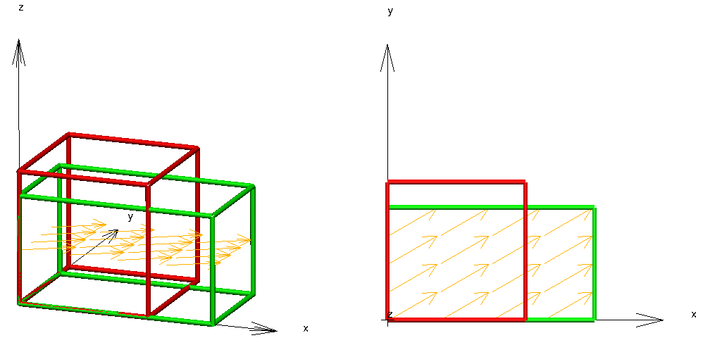
- Now consider the same deformation, except that the material fibre axes are no longer aligned with the reference spatial axes. They are now rotated anti-clockwise by an angle of \(\theta=30\) degrees from the \(X_{1}\) axis (in the \(X_{1}\)-\(X_{2}\) plane), as shown in the figure below.
For the following exercises, you are asked to transform strain and stress tensors between the reference spatial coordinates and the material fibre coordinate systems using the generalised rotational transform given by:
\[\boldsymbol{E}_{fib} = \boldsymbol{Q}^{T} \boldsymbol{E}_{ref} \boldsymbol{Q}\]where \(\boldsymbol{E}_{ref}\) and \(\boldsymbol{E}_{fib}\) are Green-Lagrange strain tensors defined with respect to the reference spatial and material fibre axes, respectively, and \(\boldsymbol{Q}\) is the orthogonal rotation matrix, which for this example is defined by:
\[\begin{split}\boldsymbol{Q} = \begin{bmatrix} \cos(\theta) & -\sin(\theta) & 0 \\ \sin(\theta) & \cos(\theta) & 0 \\ 0 & 0 & 1 \end{bmatrix}\end{split}\]
- Calculate the components of the Green-Lagrange strain tensor with respect to the material fibre axes (\(\boldsymbol{E}_{fib}\)) via the appropriate tensor transformation (see Step 3).
- Explain similarities/differences between \(\boldsymbol{E}_{fib}\) and \(\boldsymbol{E}_{ref}\) for this model.
- The relationship between second Piola-Kirchhoff stress tensors defined with respect to reference spatial and material fibre coordinates is (note the similarity to Step 3):
\[\boldsymbol{T}_{fib} = \boldsymbol{Q}^{T} \boldsymbol{T}_{ref} \boldsymbol{Q}\]Invert this equation, and then calculate the second Piola-Kirchhoff stress components with respect to the reference spatial axes (\(\boldsymbol{T}_{ref}\)) from the following components of the second Piola-Kirchhoff stress tensor with respect to the material fibre axes (\(\boldsymbol{T}_{fib}\)):
\[\begin{split}\boldsymbol{T_{fib}} = \begin{bmatrix} 330.345 & -190.725 & 0 \\ -190.725 & 110.115 & 0 \\ 0 & 0 & 0 \end{bmatrix}\end{split}\]
- Explain similarities/differences between \(\boldsymbol{T}_{fib}\) and \(\boldsymbol{T}_{ref}\) for this model.
- What would you expect from the analysis in steps 4-7 if the fibre angle was changed from \(\theta=30\) degrees to \(\theta=45\) degrees, or to \(\theta=90\) degrees for this model? Explain the differences/similarities of the stress tensors \(\boldsymbol{T}_{fib}\) and \(\boldsymbol{T}_{ref}\) for this uniaxial deformation model.
Note
You should not need to do any calculations to answer this questions, but if you would like the extra practice, perform steps 4-7 using:
\(\theta=45\) degrees, where the second Piola-Kirchhoff stress tensor with respect to the material fibre axes is:
\[\begin{split}\boldsymbol{T_{fib}} = \begin{bmatrix} 220.2 & -220.2 & 0 \\ -220.2 & 220.2 & 0 \\ 0 & 0 & 0 \end{bmatrix}\end{split}\]and/or \(\theta=90\) degrees, where the second Piola-Kirchhoff stress tensor with respect to the material fibre axes is:
\[\begin{split}\boldsymbol{T_{fib}} = \begin{bmatrix} 0 & 0 & 0 \\ 0 & 440.5 & 0 \\ 0 & 0 & 0 \end{bmatrix}\end{split}\]
Here are the solutions to Steps 1-8.
Equi-biaxial extension of a unit cube
- Start OpenCMISS and load the stress analysis project (described in the Starting OpenCMISS section).
- Select “Model 1 (Equi-biaxial extension of unit cube, 0 degree fibre rotation)” from the drop down menu and click the “Run” button (screenshots of this procedure are shown in the Running models in OpenCMISS section).
- After a short time, the model should have solved and the simulation results will appear in the 3D graphics window as shown in the screenshot below.
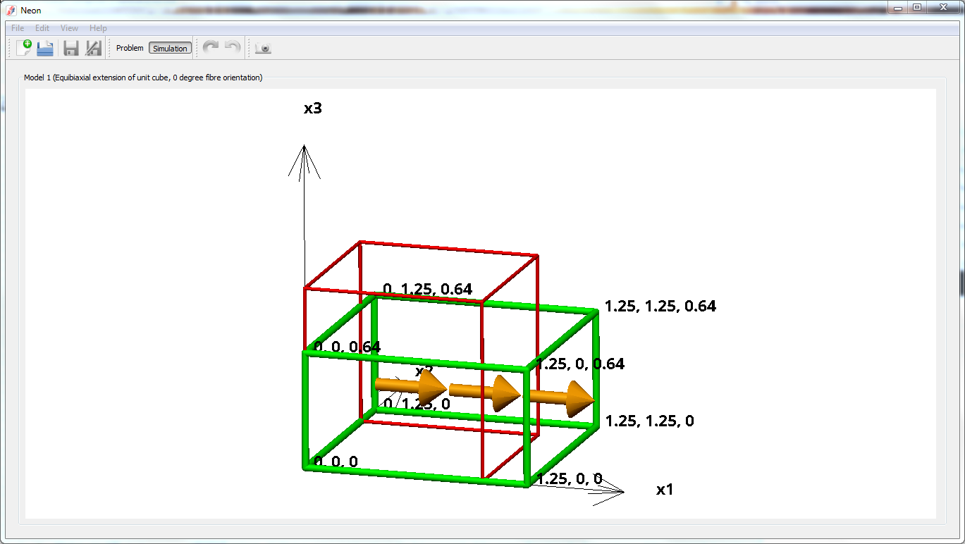
In this graphical window:
- the undeformed (reference) configuration of the unit cube is shown in red, and
- the deformed (current) configuration is shown in green (\(x_{1}\), \(x_{2}\), \(x_{3}\) components of the deformed coordinates are shown at the corners of the model.
- ignore the gold arrows for now - these will be needed later.
The model in the 3D graphics window can be rotated (click-drag-left-mouse button), translated (click-drag-middle-mouse button), or zoomed (click-drag-middle-mouse button).
- This equi-biaxial deformation is incompressible (i.e. maintains constant volume) described by the equations:
\[x_1 = \frac{5}{4}X_1 ~~~~ x_2 = \frac{5}{4}X_2 ~~~~ x_3 = \frac{16}{25}X_3\]
- Write down:
- the deformation gradient tensor (\(\boldsymbol{F}=\frac{\partial\boldsymbol{x}}{\partial\boldsymbol{X}}\)),
- the right Cauchy-Green deformation tensor (\(\boldsymbol{C}\)), and
- Green-Lagrange strain tensor (\(\boldsymbol{E}\)) (label this \(\boldsymbol{E}_{ref}\)).
Note
This is the same deformation used in Model 2 of Lab 1, so you should not need to re-do these calculations.
Equi-biaxial deformation with respect to rotated material fibre axes
- Return to the model selection drop down menu and select/run “Model 3 (Equi-biaxial extension of unit cube, 30 degree fibre rotation)”. This model is similar to the previous models, except that the material fibre axes are no longer aligned with the reference (spatial) axes. For this model, the material fibre axis is rotated anti-clockwise by an angle of \(\theta=30\) degrees from the \(X_{1}\) axis (in the \(X_{1}\)-\(X_{2}\) plane). When visualising these models, the gold arrows in the graphics window indicate the direction of the first material fibre axis (along which the first material coordinate is defined), and the second material fibre axis (not shown) is perpendicular to the gold arrow but lies within \(X_{1}\)-\(X_{2}\) plane.
- Determine the Green-Lagrange strain tensor components with respect to the material fibre axes (\(\boldsymbol{E}_{fib}\)) using the approach in Section 2.
- Check your answers to Step 15 against the simulation results from OpenCMISS.
Note
Drag the right edge of the 3D graphics window to reveal the stress and strain tensor components associated with the simulation in material fibre and reference spatial coordinates. See this link for an example on how to open this pane.
- Explain similarities/differences between \(\boldsymbol{E}_{fib}\) and \(\boldsymbol{E}_{ref}\) for this model.
- From the solution output, write down \(\boldsymbol{T}_{fib}\) (the second Piola-Kirchhoff stress tensor with respect to the material fibre axes). Use this to determine the second Piola-Kirchhoff stress components with respect to the reference spatial coordinate axes (\(\boldsymbol{T}_{ref}\)) via the approach Section 2.
- Check your answers to Step 18 against the simulation results.
- Explain similarities/differences between \(\boldsymbol{T}_{fib}\) and \(\boldsymbol{T}_{ref}\) for this model.
- What would you expect from the analysis in steps 15-20 if the fibre angle was changed from \(\theta=30\) degrees to \(\theta=45\) degrees, or to \(\theta=90\) degrees for this equi-biaxial deformation model? Explain the differences/similarities between the two strain tensors for this model. Then explain the differences/similarities between the two stress tensors for this model.
Note
You should not need to do any calculations to answer this questions. It is fine to do so if you would like some extra practice - just perform steps 15-20 with \(\theta=45\) degrees by selecting the Model 4 then Model 6 from the “Run” menu.
Here are the solutions to Step 21.
Questions to think about:
After you have completed the exercises above, consider the following questions:
- How do changes in \(\boldsymbol{E}_{ref}\) for different fibre angles (\(\theta\)) in the equi-biaxial deformation compare with the changes seen in the uniaxial deformation.
- How do changes in \(\boldsymbol{E}_{fib}\) for different fibre angles (\(\theta\)) in the equi-biaxial deformation compare with the changes seen in the uniaxial deformation.
- How do changes in \(\boldsymbol{T}_{ref}\) for different fibre angles (\(\theta\)) in the equi-biaxial deformation compare with the changes seen in the uniaxial deformation.
- How do changes in \(\boldsymbol{T}_{fib}\) for different fibre angles (\(\theta\)) in the equi-biaxial deformation compare with the changes seen in the uniaxial deformation.
- Will the invariants of \(\boldsymbol{C}\) be the same or different when calculated with respect to reference spatial or material fibre coordinates?
Note
By completing this lab, you should be able to:
- convert between 2nd Piola-Kirchhoff and Cauchy stress tensors.
- analyse large deformation kinematics with respect to reference spatial or rotated material fibre coordinates, and convert between them.
- analyse stress tensors with respect to reference spatial or rotated material fibre coordinates, and convert between them.